母平均の比較値との差のz検定
- sympyとscipyで試してみる
- statsmodels
- R
In [1]:
%matplotlib inline

import numpy as np
import pandas as pd
from scipy import stats
import matplotlib.pyplot as plt
import statsmodels.api as sm
import seaborn as sns
import sympy
from sympy import symbols, Symbol, Rational
In [2]:
import sys
print(sys.version)
3.5.2 |Anaconda custom (x86_64)| (default, Jul  2 2016, 17:52:12)
[GCC 4.2.1 Compatible Apple LLVM 4.2 (clang-425.0.28)]
In [3]:
%load_ext rpy2.ipython
In [4]:
import rpy2
rpy2.__version__
Out[4]:
'2.8.5'
In [5]:
!R --version
R version 3.4.0 (2017-04-21) -- "You Stupid Darkness"
Copyright (C) 2017 The R Foundation for Statistical Computing
Platform: x86_64-apple-darwin15.6.0 (64-bit)

R is free software and comes with ABSOLUTELY NO WARRANTY.
You are welcome to redistribute it under the terms of the
GNU General Public License versions 2 or 3.
For more information about these matters see
http://www.gnu.org/licenses/.
In [6]:
sympy.init_printing()
データ準備
In [7]:
np.random.seed(0)
mean = 1183000
std = 101000
size = 250
other_mean = 1150000
x = np.random.normal(size=size)
x.mean(), x.std()
Out[7]:
$$\left ( 0.0317806978638, \quad 0.99610052371\right )$$
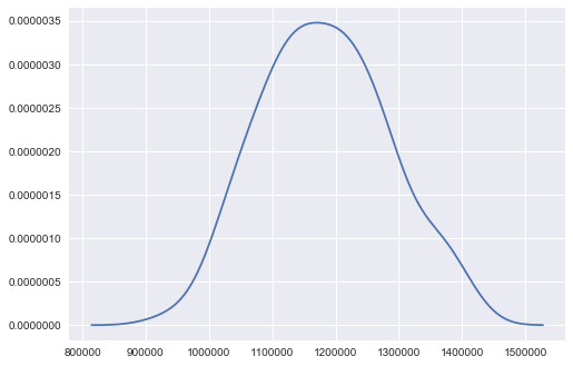
平均と標準偏差を調整する
In [8]:
x1 = x / x.std() * std
x1 = x1 + (mean - x1.mean())
x1.mean(), x1.std()
Out[8]:
$$\left ( 1183000.0, \quad 101000.0\right )$$
In [9]:
x2 = x + (other_mean - x.mean())
x2.mean(), x2.std()
Out[9]:
$$\left ( 1150000.0, \quad 0.996100523709\right )$$
In [10]:
sns.kdeplot(x1)
Out[10]:
<matplotlib.axes._subplots.AxesSubplot at 0x115a4d518>
検定統計量
In [11]:
x_, μ0, σ, n = symbols("\overline{x} mu_0 sigma n")
x_, μ0, σ, n
Out[11]:
$$\left ( \overline{x}, \quad \mu_{0}, \quad \sigma, \quad n\right )$$
In [12]:
T = (x_ -  μ0) / (σ / sympy.sqrt(n))
T
Out[12]:
$$\frac{\sqrt{n}}{\sigma} \left(\overline{x} - \mu_{0}\right)$$
symbolを用意して式を組み立てたが、定義どおりの形にならない
In [13]:
sympy.S("x - mu_0")
Out[13]:
$$- \mu_{0} + x$$
In [14]:
#sympy.S("overline{x} + 1")
- アルファベット順のため定義どおりの順序にならない
- latexの一部は自由に使えない
In [15]:
T = sympy.S("(X_overline - mu_0) / (sigma / sqrt(n))", evaluate=False)
T
Out[15]:
$$\frac{X_{overline} - \mu_{0}}{\sigma \frac{1}{\sqrt{n}}}$$
妥協して順序を考慮した式の組み立てに成功
検定統計量の算出
書籍と同じ値になることの確認
In [16]:
T_value = T.subs(
    dict(
        X_overline=mean,
        mu_0=other_mean,
        sigma=std,
        n=size)).evalf()
T_value
Out[16]:
$$5.16609716760181$$
有意水準0.05片側での統計量の確認
有意であるか確認
In [17]:
stats.norm.ppf(1 - 0.05)
Out[17]:
$$1.64485362695$$
書籍と同じ値で確認
In [18]:
stats.norm.sf(5.17)
Out[18]:
$$1.17046997373e-07$$
In [19]:
1 - stats.norm.cdf(float(T_value))
Out[19]:
$$1.19516280317e-07$$
不偏の場合?の確認
In [20]:
T_value_n_1 = T.subs(
    dict(
        X_overline=mean,
        mu_0=other_mean,
        sigma=std,
        n=size-1)).evalf()
T_value_n_1
Out[20]:
$$5.15575462035607$$
In [21]:
1 - stats.norm.cdf(float(T_value_n_1))
Out[21]:
$$1.26305760739e-07$$
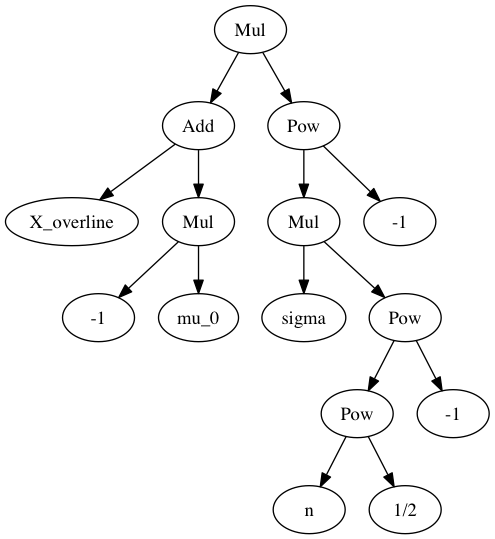
(おまけ)Sympyの式のグラフ化
In [22]:
sympy.srepr(T)
Out[22]:
"Mul(Pow(Mul(Symbol('sigma'), Pow(Pow(Symbol('n'), Rational(1, 2)), Integer(-1))), Integer(-1)), Add(Symbol('X_overline'), Mul(Integer(-1), Symbol('mu_0'))))"
In [23]:
from sympy.printing.dot import dotprint
import pydot_ng
from IPython.display import Image

graph = pydot_ng.graph_from_dot_data(dotprint(T))
Image(graph.create_png())
Out[23]:
statsmodels
3とおり
- ztest function
- descriptive statistics and tests with weights for case weights
- class for two sample comparison (2を利用)
1. ztest function
http://www.statsmodels.org/stable/generated/statsmodels.stats.weightstats.ztest.html
- データセット1つとその他の平均値
- データセット2つ
In [24]:
sm.stats.ztest(x1, alternative="larger", value=other_mean)
Out[24]:
$$\left ( 5.15575462036, \quad 1.26305760785e-07\right )$$
In [25]:
sm.stats.ztest(x1, x2=x2, alternative="larger")
Out[25]:
$$\left ( 5.15575462011, \quad 1.26305760954e-07\right )$$
自由度の変更
In [26]:
sm.stats.ztest(x1, alternative="larger", value=other_mean, ddof=0)
Out[26]:
$$\left ( 5.1660971676, \quad 1.19516280322e-07\right )$$
2. descriptive statistics and tests with weights for case weights
http://www.statsmodels.org/stable/generated/statsmodels.stats.weightstats.DescrStatsW.html
In [27]:
d1 = sm.stats.DescrStatsW(x1)
d2 = sm.stats.DescrStatsW(x2)
d1
Out[27]:
<statsmodels.stats.weightstats.DescrStatsW at 0x11878cd30>
In [28]:
d1.ztest_mean(other_mean, alternative="larger")
Out[28]:
$$\left ( 5.15575462036, \quad 1.26305760785e-07\right )$$
3. class for two sample comparison (2を利用)
http://www.statsmodels.org/devel/generated/statsmodels.stats.weightstats.CompareMeans.html
In [29]:
compare_means = sm.stats.CompareMeans(d1, d2)
compare_means
Out[29]:
<statsmodels.stats.weightstats.CompareMeans at 0x11878cb38>
In [30]:
compare_means.ztest_ind(alternative="larger")
Out[30]:
$$\left ( 5.15575462011, \quad 1.26305760954e-07\right )$$
R
z.testはなかったので、単純に計算
- http://rpy.sourceforge.net/rpy2/doc-2.4/html/interactive.html
- https://www.slideshare.net/Prunus1350/5-r-14210894
In [31]:
%%R -i x1 --input std -i size -i other_mean --output r2py_output

Z分子 <- mean(x1) - other_mean
Z分母 <- std / sqrt(size)
Z統計量 <- Z分子 / Z分母
p値 <- pnorm(Z統計量, lower.tail = FALSE)
r2py_output <- c(Z統計量, p値)
r2py_output
[1] 5.166097e+00 1.195163e-07
In [32]:
r2py_output
Out[32]:
array([ 5.16609717e+00, 1.19516280e-07])
下記を参考にscipyとの対応を確認できるようにしておく
http://cse.naro.affrc.go.jp/takezawa/r-tips/r/60.html
In [33]:
%%R

# for help
?dnorm
R Help on ‘dnorm’Normal                  package:stats                  R Documentation

_T_h_e _N_o_r_m_a_l _D_i_s_t_r_i_b_u_t_i_o_n

_D_e_s_c_r_i_p_t_i_o_n:

     Density, distribution function, quantile function and random
     generation for the normal distribution with mean equal to ‘mean’
     and standard deviation equal to ‘sd’.

_U_s_a_g_e:

     dnorm(x, mean = 0, sd = 1, log = FALSE)
     pnorm(q, mean = 0, sd = 1, lower.tail = TRUE, log.p = FALSE)
     qnorm(p, mean = 0, sd = 1, lower.tail = TRUE, log.p = FALSE)
     rnorm(n, mean = 0, sd = 1)

_A_r_g_u_m_e_n_t_s:

    x, q: vector of quantiles.

       p: vector of probabilities.

       n: number of observations. If ‘length(n) > 1’, the length is
          taken to be the number required.

    mean: vector of means.

      sd: vector of standard deviations.

log, log.p: logical; if TRUE, probabilities p are given as log(p).

lower.tail: logical; if TRUE (default), probabilities are P[X <= x]
          otherwise, P[X > x].

_D_e_t_a_i_l_s:

     If ‘mean’ or ‘sd’ are not specified they assume the default
     values of ‘0’ and ‘1’, respectively.

     The normal distribution has density

            f(x) = 1/(sqrt(2 pi) sigma) e^-((x - mu)^2/(2 sigma^2))

     where mu is the mean of the distribution and sigma the standard
     deviation.

_V_a_l_u_e:

     ‘dnorm’ gives the density, ‘pnorm’ gives the distribution
     function, ‘qnorm’ gives the quantile function, and ‘rnorm’
     generates random deviates.

     The length of the result is determined by ‘n’ for ‘rnorm’, and
     is the maximum of the lengths of the numerical arguments for the
     other functions.

     The numerical arguments other than ‘n’ are recycled to the
     length of the result.  Only the first elements of the logical
     arguments are used.

     For ‘sd = 0’ this gives the limit as ‘sd’ decreases to 0, a
     point mass at ‘mu’.  ‘sd < 0’ is an error and returns ‘NaN’.

_S_o_u_r_c_e:

     For ‘pnorm’, based on

     Cody, W. D. (1993) Algorithm 715: SPECFUN - A portable FORTRAN
     package of special function routines and test drivers.  _ACM
     Transactions on Mathematical Software_ *19*, 22-32.

     For ‘qnorm’, the code is a C translation of

     Wichura, M. J. (1988) Algorithm AS 241: The percentage points of
     the normal distribution.  _Applied Statistics_, *37*, 477-484.

     which provides precise results up to about 16 digits.

     For ‘rnorm’, see RNG for how to select the algorithm and for
     references to the supplied methods.

_R_e_f_e_r_e_n_c_e_s:

     Becker, R. A., Chambers, J. M. and Wilks, A. R. (1988) _The New S
     Language_.  Wadsworth & Brooks/Cole.

     Johnson, N. L., Kotz, S. and Balakrishnan, N. (1995) _Continuous
     Univariate Distributions_, volume 1, chapter 13.  Wiley, New York.

_S_e_e _A_l_s_o:

     Distributions for other standard distributions, including
     ‘dlnorm’ for the _Log_normal distribution.

_E_x_a_m_p_l_e_s:

     require(graphics)

     dnorm(0) == 1/sqrt(2*pi)
     dnorm(1) == exp(-1/2)/sqrt(2*pi)
     dnorm(1) == 1/sqrt(2*pi*exp(1))

     ## Using "log = TRUE" for an extended range :
     par(mfrow = c(2,1))
     plot(function(x) dnorm(x, log = TRUE), -60, 50,
          main = "log { Normal density }")
     curve(log(dnorm(x)), add = TRUE, col = "red", lwd = 2)
     mtext("dnorm(x, log=TRUE)", adj = 0)
     mtext("log(dnorm(x))", col = "red", adj = 1)

     plot(function(x) pnorm(x, log.p = TRUE), -50, 10,
          main = "log { Normal Cumulative }")
     curve(log(pnorm(x)), add = TRUE, col = "red", lwd = 2)
     mtext("pnorm(x, log=TRUE)", adj = 0)
     mtext("log(pnorm(x))", col = "red", adj = 1)

     ## if you want the so-called 'error function'
     erf <- function(x) 2 * pnorm(x * sqrt(2)) - 1
     ## (see Abramowitz and Stegun 29.2.29)
     ## and the so-called 'complementary error function'
     erfc <- function(x) 2 * pnorm(x * sqrt(2), lower = FALSE)
     ## and the inverses
     erfinv <- function (x) qnorm((1 + x)/2)/sqrt(2)
     erfcinv <- function (x) qnorm(x/2, lower = FALSE)/sqrt(2)
In [34]:
%%R
norm_list <- list()

set.seed(0)

norm_list[["pdf_dnorm"]] <- dnorm(5.17)
norm_list[["cdf_pnrom_T"]] <- pnorm(5.17, lower.tail = T)
norm_list[["cdf_pnrom_F"]] <- pnorm(5.17, lower.tail = F)
norm_list[["quantile_qnorm_T"]] <- qnorm(0.05, lower.tail = T)
norm_list[["quantile_qnorm_F"]] <- qnorm(0.05, lower.tail = F)
norm_list[["random_variable_rnorm"]] <- rnorm(n=10, mean=5, sd=10)

norm_list

#      dnorm(x, mean = 0, sd = 1, log = FALSE)
#      pnorm(q, mean = 0, sd = 1, lower.tail = TRUE, log.p = FALSE)
#      qnorm(p, mean = 0, sd = 1, lower.tail = TRUE, log.p = FALSE)
#      rnorm(n, mean = 0, sd = 1)
$pdf_dnorm
[1] 6.263299e-07

$cdf_pnrom_T
[1] 0.9999999

$cdf_pnrom_F
[1] 1.17047e-07

$quantile_qnorm_T
[1] -1.644854

$quantile_qnorm_F
[1] 1.644854

$random_variable_rnorm
 [1]  17.629543   1.737666  18.297993  17.724293   9.146414 -10.399500
 [7]  -4.285670   2.052796   4.942328  29.046534
In [ ]: