LogisticRegression

import numpy as np
import matplotlib.pyplot as plt
import seaborn as sns
import pandas as pd

%matplotlib inline

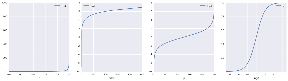
オッズとlogit

• p / (1- p)
• 上記に対数関数適用

def odds(p):
    return p / (1 - p)

def plot_logit(ps):
    figure, axes = plt.subplots(1, 4, figsize=(20, 5))

    s_odds = np.vectorize(odds)(ps)
    s_logit = np.log(s_odds)
    df = pd.DataFrame({
            "p": ps,
            "odds": s_odds,
            "logit": s_logit
        })
    df.plot(x="p", y="odds", ax=axes[0])
    df.plot(x="odds", y="logit", ax=axes[1])
    df.plot(x="p", y="logit", ax=axes[2])
    df.plot(y="p", x="logit", ax=axes[3])

    return df.T

plot_logit(np.linspace(0.001, 0.999, 999))

	0	1	2	3	4	5	6	7	8	9	...	989	990	991	992	993	994	995	996	997	998
logit	-6.906755	-6.212606	-5.806138	-5.517453	-5.293305	-5.109978	-4.954821	-4.820282	-4.701490	-4.595120	...	4.59512	4.701490	4.820282	4.954821	5.109978	5.293305	5.517453	5.806138	6.212606	6.906755
odds	0.001001	0.002004	0.003009	0.004016	0.005025	0.006036	0.007049	0.008065	0.009082	0.010101	...	99.00000	110.111111	124.000000	141.857143	165.666667	199.000000	249.000000	332.333333	499.000000	999.000000
p	0.001000	0.002000	0.003000	0.004000	0.005000	0.006000	0.007000	0.008000	0.009000	0.010000	...	0.99000	0.991000	0.992000	0.993000	0.994000	0.995000	0.996000	0.997000	0.998000	0.999000

3 rows × 999 columns

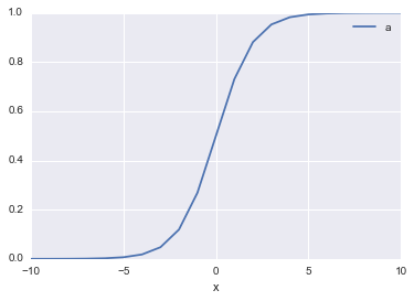
logitの逆関数(ロジスティック関数)

• y = log(p/ (1 - p))
• -y = log((1 - p) / p) = log(1/p - 1)
• exp(-y) = (1/p - 1)
• exp(-y) + 1 = 1/p
• p = 1 / (exp(-y) + 1)

http://www012.upp.so-net.ne.jp/doi/biostat/CT39/glm.pdf

def a(x):
    return 1.0 / (1.0 + np.exp(-x))

def plot_a(xs):
    s_a = np.vectorize(a)(xs)
    df = pd.DataFrame({
            "x": xs,
            "a": s_a
        })
    df.plot(x="x", y="a")

    return df.T

plot_a(np.arange(-10, 11))

	0	1	2	3	4	5	6	7	8	9	...	11	12	13	14	15	16	17	18	19	20
a	0.000045	0.000123	0.000335	0.000911	0.002473	0.006693	0.017986	0.047426	0.119203	0.268941	...	0.731059	0.880797	0.952574	0.982014	0.993307	0.997527	0.999089	0.999665	0.999877	0.999955
x	-10.000000	-9.000000	-8.000000	-7.000000	-6.000000	-5.000000	-4.000000	-3.000000	-2.000000	-1.000000	...	1.000000	2.000000	3.000000	4.000000	5.000000	6.000000	7.000000	8.000000	9.000000	10.000000

2 rows × 21 columns