datascientist_mook_vol1¶

データサイエンティスト養成読本vol.1（Python 機械学習）¶

In [1]:

import numpy as np
import pandas as pd
import matplotlib.pyplot as plt
import seaborn as sns

%matplotlib inline

irisデータ読み込み(from pandas repogitory)¶

In [2]:

import os

iris_pandas_url = "https://raw.githubusercontent.com/pydata/pandas/master/doc/data/iris.data"
iris_data_file_name = "iris.data.csv"
if os.path.exists(iris_data_file_name):
    iris = pd.read_csv(iris_data_file_name)
else:
    iris = pd.read_csv(iris_pandas_url)
    iris.to_csv(iris_data_file_name, index=False)
iris.info()

<class 'pandas.core.frame.DataFrame'>
RangeIndex: 150 entries, 0 to 149
Data columns (total 5 columns):
SepalLength    150 non-null float64
SepalWidth     150 non-null float64
PetalLength    150 non-null float64
PetalWidth     150 non-null float64
Name           150 non-null object
dtypes: float64(4), object(1)
memory usage: 5.9+ KB

In [3]:

setosa = iris[iris.Name == "Iris-setosa"]
versicolor = iris[iris.Name == "Iris-versicolor"]
virginica = iris[iris.Name == "Iris-virginica"]
len(setosa), len(versicolor), len(virginica),

Out[3]:

(50, 50, 50)

In [4]:

iris.pivot_table(index="Name", aggfunc=np.mean)

Out[4]:

	PetalLength	PetalWidth	SepalLength	SepalWidth
Name
Iris-setosa	1.464	0.244	5.006	3.418
Iris-versicolor	4.260	1.326	5.936	2.770
Iris-virginica	5.552	2.026	6.588	2.974

In [5]:

pd.concat(
    [
        setosa.sum(),
        setosa.mean(), setosa.median(),
        setosa.min(), setosa.max(),
        setosa.var(), setosa.std(),
    ], axis=1,
    keys=["sum", "mean", "median", "min", "max", "var", "std"]
)

Out[5]:

	sum	mean	median	min	max	var	std
Name	Iris-setosaIris-setosaIris-setosaIris-setosaIr...	NaN	NaN	Iris-setosa	Iris-setosa	NaN	NaN
PetalLength	73.2	1.464	1.5	1	1.9	0.030106	0.173511
PetalWidth	12.2	0.244	0.2	0.1	0.6	0.011494	0.107210
SepalLength	250.3	5.006	5.0	4.3	5.8	0.124249	0.352490
SepalWidth	170.9	3.418	3.4	2.3	4.4	0.145180	0.381024

In [6]:

setosa.describe().T

Out[6]:

	count	mean	std	min	25%	50%	75%	max
SepalLength	50.0	5.006	0.352490	4.3	4.800	5.0	5.200	5.8
SepalWidth	50.0	3.418	0.381024	2.3	3.125	3.4	3.675	4.4
PetalLength	50.0	1.464	0.173511	1.0	1.400	1.5	1.575	1.9
PetalWidth	50.0	0.244	0.107210	0.1	0.200	0.2	0.300	0.6

In [7]:

[
    np.arange(0, 1.1, 0.1),
    np.linspace(0, 1, 11)
]

Out[7]:

[array([ 0. ,  0.1,  0.2,  0.3,  0.4,  0.5,  0.6,  0.7,  0.8,  0.9,  1. ]),
 array([ 0. ,  0.1,  0.2,  0.3,  0.4,  0.5,  0.6,  0.7,  0.8,  0.9,  1. ])]

In [8]:

setosa.describe(include="all", percentiles=np.linspace(0.1, 0.9, 9)).T

Out[8]:

	count	unique	top	freq	mean	std	min	10%	20%	30.0%	40%	50%	60%	70%	80%	90%	max
SepalLength	50	NaN	NaN	NaN	5.006	0.35249	4.3	4.59	4.7	4.8	4.96	5	5.1	5.1	5.32	5.41	5.8
SepalWidth	50	NaN	NaN	NaN	3.418	0.381024	2.3	3	3.1	3.2	3.36	3.4	3.5	3.53	3.72	3.9	4.4
PetalLength	50	NaN	NaN	NaN	1.464	0.173511	1	1.3	1.3	1.4	1.4	1.5	1.5	1.5	1.6	1.7	1.9
PetalWidth	50	NaN	NaN	NaN	0.244	0.10721	0.1	0.1	0.2	0.2	0.2	0.2	0.2	0.3	0.3	0.4	0.6
Name	50	1	Iris-setosa	50	NaN	NaN	NaN	NaN	NaN	NaN	NaN	NaN	NaN	NaN	NaN	NaN	NaN

In [9]:

setosa.corr()

Out[9]:

	SepalLength	SepalWidth	PetalLength	PetalWidth
SepalLength	1.000000	0.746780	0.263874	0.279092
SepalWidth	0.746780	1.000000	0.176695	0.279973
PetalLength	0.263874	0.176695	1.000000	0.306308
PetalWidth	0.279092	0.279973	0.306308	1.000000

In [10]:

setosa.cov()

Out[10]:

	SepalLength	SepalWidth	PetalLength	PetalWidth
SepalLength	0.124249	0.100298	0.016139	0.010547
SepalWidth	0.100298	0.145180	0.011682	0.011437
PetalLength	0.016139	0.011682	0.030106	0.005698
PetalWidth	0.010547	0.011437	0.005698	0.011494

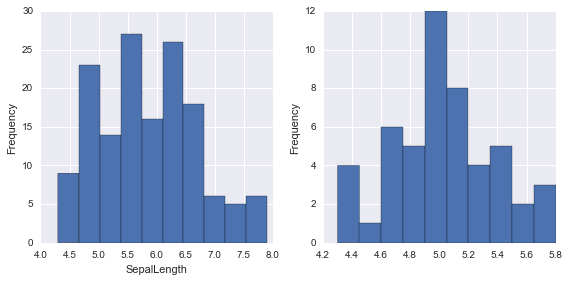
In [11]:

fig, axes = plt.subplots(1, 2, figsize=(8, 4))
iris.SepalLength.plot.hist(ax=axes[0])
axes[0].set_xlabel("SepalLength")

setosa.SepalLength.plot.hist(ax=axes[1])

plt.tight_layout()

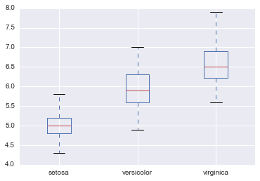
../../../_images/contents_notebooks_books_datascientist_mook_vol1_12_0.png

In [12]:

pd.concat(
    {
        "setosa": setosa.SepalLength,
        "versicolor": versicolor.SepalLength,
        "virginica": virginica.SepalLength
    }, axis=1
).plot.box()

Out[12]:

<matplotlib.axes._subplots.AxesSubplot at 0x117375e10>

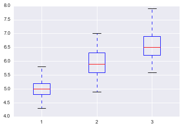
../../../_images/contents_notebooks_books_datascientist_mook_vol1_13_1.png

In [13]:

data = [setosa.SepalLength, versicolor.SepalLength, virginica.SepalLength]
plt.boxplot(data)
"dummy"

Out[13]:

'dummy'

../../../_images/contents_notebooks_books_datascientist_mook_vol1_14_1.png

In [14]:

setosa.plot.scatter(x="SepalLength",y="SepalWidth")

Out[14]:

<matplotlib.axes._subplots.AxesSubplot at 0x119eff4e0>

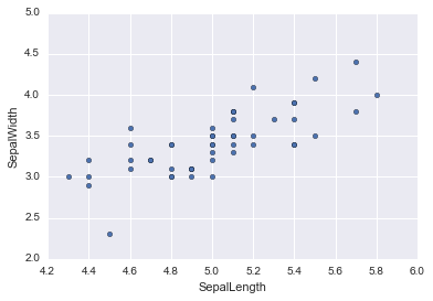
../../../_images/contents_notebooks_books_datascientist_mook_vol1_15_1.png

In [15]:

setosa.corr().ix["SepalLength", "SepalWidth"]

Out[15]:

0.74678037326392688

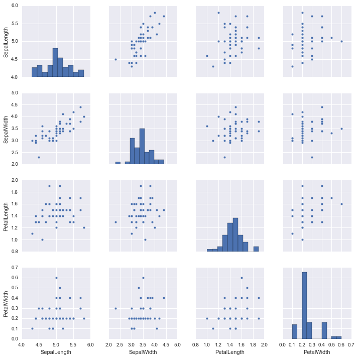
In [16]:

sns.pairplot(setosa)
plt.tight_layout()

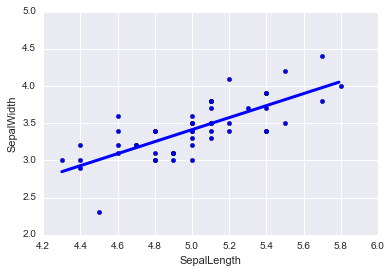
../../../_images/contents_notebooks_books_datascientist_mook_vol1_17_0.png

In [17]:

from sklearn import linear_model
np.random.seed(0)

linear_regr = linear_model.LinearRegression()
X = setosa[["SepalLength"]]
Y = setosa[["SepalWidth"]]
linear_regr.fit(X, Y)

plt.scatter(X, Y)
# http://sucrose.hatenablog.com/entry/2013/03/16/162019
px = np.arange(X.min(), X.max(), 0.01)[:, np.newaxis]
py = linear_regr.predict(px)
# print(px.shape, py.shape)

plt.plot(px, py, color="blue", linewidth=3)
plt.xlabel("SepalLength")
plt.ylabel("SepalWidth")

linear_regr.coef_, linear_regr.intercept_, linear_regr.score(X, Y)

Out[17]:

(array([[ 0.80723367]]), array([-0.62301173]), 0.55768092589220974)

../../../_images/contents_notebooks_books_datascientist_mook_vol1_18_1.png

In [18]:

linear_regr = linear_model.LinearRegression()
X = setosa[["SepalLength", "PetalLength", "PetalWidth"]]
Y = setosa[["SepalWidth"]]
linear_regr.fit(X, Y)
linear_regr.coef_, linear_regr.intercept_, linear_regr.score(X, Y)

Out[18]:

(array([[ 0.79303981, -0.09677873,  0.31530122]]),
 array([-0.48720671]),
 0.56492621264573206)

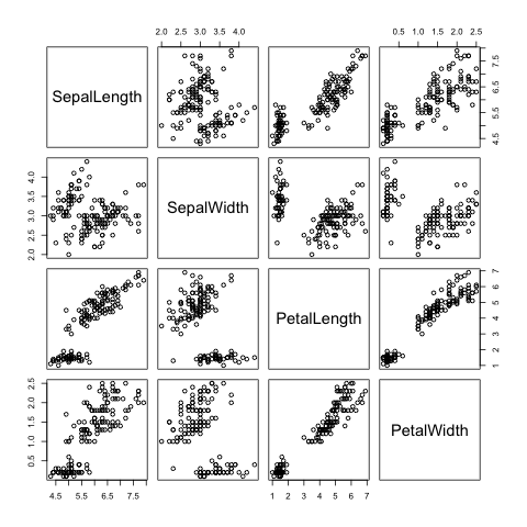
In [20]:

import pyper
import os

image_file_name = "image.png"
r_source = """library(dplyr)
png("{0}", width = 480, height = 480, pointsize = 12, bg = "white", res = NA)
pairs(select(r_data, c(-Name)))
dev.off()
""".format(image_file_name)

r = pyper.R(use_pandas = "True")
r_source_file = "example.R"
r.assign("r_data", iris)
print(r("summary(r_data)"))

with open(r_source_file, "w", encoding="sjis") as f:
    f.write(r_source)
print(r("source(file='{}')".format(r_source_file)))
os.remove(r_source_file)

from IPython.core.display import Image
Image(image_file_name)
#os.remove(image_file_name)

try({summary(r_data)})
  SepalLength      SepalWidth     PetalLength      PetalWidth
 Min.   :4.300   Min.   :2.000   Min.   :1.000   Min.   :0.100
 1st Qu.:5.100   1st Qu.:2.800   1st Qu.:1.600   1st Qu.:0.300
 Median :5.800   Median :3.000   Median :4.350   Median :1.300
 Mean   :5.843   Mean   :3.054   Mean   :3.759   Mean   :1.199
 3rd Qu.:6.400   3rd Qu.:3.300   3rd Qu.:5.100   3rd Qu.:1.800
 Max.   :7.900   Max.   :4.400   Max.   :6.900   Max.   :2.500
              Name
 Iris-setosa    :50
 Iris-versicolor:50
 Iris-virginica :50




<pyper.R object at 0x11b7455f8>
try({source(file='example.R')})

 次のパッケージを付け加えます: ‘dplyr’

 以下のオブジェクトは ‘package:stats’ からマスクされています:

     filter, lag

 以下のオブジェクトは ‘package:base’ からマスクされています:

     intersect, setdiff, setequal, union

Out[20]:

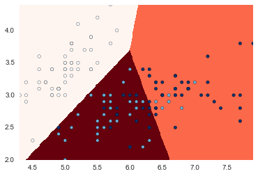
../../../_images/contents_notebooks_books_datascientist_mook_vol1_20_1.png

In [25]:

# k-means
def category2int(x):
    category = {
        "Iris-setosa": 0,
        "Iris-versicolor": 1,
        "Iris-virginica": 2,
    }
    return category[x]

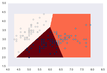
In [45]:

from sklearn.cluster import KMeans

X = iris[["SepalLength", "SepalWidth"]]
kmeansCls = KMeans(n_clusters=3)
kmeansCls.fit(X)

[print(a, "\n", getattr(kmeansCls, a)) for a in dir(kmeansCls) if not a.startswith("_") and a.endswith("_")]

Y = iris.Name.map(category2int)
xMin = X.SepalLength.min()
xMax = X.SepalLength.max()
yMin = X.SepalWidth.min()
yMax = X.SepalWidth.max()
xx, yy = np.meshgrid(np.arange(xMin, xMax, 0.01), np.arange(yMin, yMax, 0.01))
Z = kmeansCls.predict(np.c_[xx.ravel(), yy.ravel()]).reshape(xx.shape)

plt.xlim(xx.min(), xx.max())
plt.ylim(yy.min(), yy.max())
plt.pcolormesh(xx, yy, Z, cmap=plt.cm.Reds)
plt.scatter(X.SepalLength, X.SepalWidth, c=np.array(Y), cmap=plt.cm.Blues)

cluster_centers_
 [[ 5.006       3.418     ]
 [ 6.81276596  3.07446809]
 [ 5.77358491  2.69245283]]
inertia_
 37.1237021277
labels_
 [0 0 0 0 0 0 0 0 0 0 0 0 0 0 0 0 0 0 0 0 0 0 0 0 0 0 0 0 0 0 0 0 0 0 0 0 0
 0 0 0 0 0 0 0 0 0 0 0 0 0 1 1 1 2 1 2 1 2 1 2 2 2 2 2 2 1 2 2 2 2 2 2 2 2
 1 1 1 1 2 2 2 2 2 2 2 2 1 2 2 2 2 2 2 2 2 2 2 2 2 2 1 2 1 1 1 1 2 1 1 1 1
 1 1 2 2 1 1 1 1 2 1 2 1 2 1 1 2 2 1 1 1 1 1 2 2 1 1 1 2 1 1 1 2 1 1 1 2 1
 1 2]
n_iter_
 6

Out[45]:

<matplotlib.collections.PathCollection at 0x11cebd710>

../../../_images/contents_notebooks_books_datascientist_mook_vol1_22_2.png

In [47]:

plt.pcolormesh(xx, yy, Z, cmap=plt.cm.Reds)
plt.scatter(X.SepalLength, X.SepalWidth, c=kmeansCls.labels_, cmap=plt.cm.Blues)

Out[47]:

<matplotlib.collections.PathCollection at 0x11afeb940>

../../../_images/contents_notebooks_books_datascientist_mook_vol1_23_1.png

In [42]:

kmeansCls.predict(np.c_[xx.ravel(), yy.ravel()])

Out[42]:

array([1, 1, 1, ..., 0, 0, 0], dtype=int32)

In [ ]:

In [ ]: